Realistic Backtester for Perpetual Futures (Part 1/2) (With Code)

A guide to writing a realistic market simulator for Crypto perpetual futures.

Table of Contents

Part 1:

• Introduction

• Simulator/backtester architecture

• Preparing the data

• Simulating a single market

• Simulating market orders

Part 2:

• Simulating trading costs

• Simulating funding

• Simulating many markets

• Finish

• Subscriber materials (source code)

Introduction

In the last article, we looked at how markets work and at simulating them in theory.

Today we will write a complete event-driven simulator/backtester for Cryptocurrency perpetual futures using historical price and funding data.

We will apply the cost model released in the last article to make the simulations realistic and useful.

The simulator and the cost model were developed in-house and are adapted from my own Quant practice to simulate/backtest trades and validate real-life results. They mimic the real world closely despite the limitations of candle data.

The complete source code is available for paying subscribers at the end of the article.

In keeping with the promise of suitability for independent practitioners, the simulator is small, at about 600 lines of code.

The article is split into two parts released on the same day. Part 1 deals with simulating a market costlessly and is free to read for everybody. Part 2 is available for paying subscribers and extends the simulator with the cost model, funding, and support for multiple markets.

Let's begin.¹²

Simulator Architecture

I will try to keep this section short since we already talked a little about it in the previous article and I want to leave more space for the meat of the article later.

The kind of simulator we will write is typically called an event-driven simulator. This is a widely used architecture that is simple and robust. I'll be using the example of Crypto perpetual futures (swaps) markets, but the architecture is universal and useful for spot, HFT, or any other trading activity that involves reacting to events.

I will try to explain it by way of example:

A quantitative trading system running live can be written generally as a function of some state and an incoming event that produces the next state to be used with the next event:

\(f(S_{n},E) \rightarrow S_{n+1}\)

We could say that the system is 'driven' by events. We saw this in prior articles in the form of a trading loop that looked something like this:

let exchange = SimulatedExchange::new(...);
let state = ...

while let Some(event) = exchange.next_event() {
    state.on_event(&event);
    ...
}

This should give you an idea of what we will write in the article. It will be a simulated exchange, which will take historical data and turn it into a stream of events used to drive a trading system/loop and simulate any other effects needed along the way, such as funding and orders.

One of the primary advantages of this model is that it allows us to use the same infrastructure for trading live and simulating. We simply replace the exchange from a simulated one to a live one to run the same code live as in the simulation. This in turn helps with validation between live and simulated environments (in either direction), helps us catch bugs and decreases the amount of work we need to do.

I wrote about this and other advantages in the previous article already so I will stop here and we will go straight to the implementation.

Preparing The Data

We begin with the data. Since we're looking at perpetual swaps (futures), we will use price data in the form of candles and funding data. We will start with the former and address funding in Part 2.

For the price, we will use regular OHLC candles. The candles I use in the code look like the one below:

pub struct Candle {
    pub open_time: i64,
    pub open: f64,
    pub high: f64,
    pub low: f64,
    pub close: f64,
    pub close_time: i64,
}

We are free to augment this with extra fields such as volume, turnover, number of trades, etc. that are frequently included with candle data. I use this particular format only for simplicity. Later in the article, we will see that we only need close and close time, and optionally the open to perform the simulation.

Funding mechanisms and data differ from exchange to exchange but it generally boils down to a fraction of a position's value being paid by or to the position holder. For our purposes, we will use the following struct representing the time when funding took place and the funding rate:

pub struct Funding {
    pub time: i64,
    pub rate: f64,
}

Price and funding data can be downloaded from exchanges for free via exchange APIs or bought from data providers such as Tardis. I have shown how to do the former in a prior article on the Exchange Client so I won't discuss it here.

To simulate a market we will need to iterate (based on a clock) on this data from oldest to latest and do some processing on each step. This will consist of emitting events, filling orders, and simulating funding. We will look at this gradually in the coming sections but first, we’ll want to figure out how to handle the data in our code.

In an earlier article, we introduced a highly performant and memory-efficient time-series storage module. Readers who have access to it should use it here. It will make our backtests much faster, and we won't be required to fit all of our data in memory, which can be a problem when we have a lot of it.

To keep things workable for everybody else, I will use a regular Vec in the examples below.

Our data per market will be two sorted arrays/buffers:

struct Buffer<T> = ...; // Assume custom type from the time-series storage article or Vec<T>.

struct MarketData {
    candles: Buffer<Candle>,
    funding: Buffer<Funding>,
}

Acquiring and loading the data was covered in prior articles so I will skip it here and go straight to simulating.

Simulating A Single Market

We will take things piecemeal and begin by simulating a single market. By the end of the article, we will extend this to multiple/all markets on an exchange.

For a realistic and useful simulation, we need to implement:

1. Price

2. Market orders

3. Trading costs

4. Funding

We start with price.

We'll want to iterate on the candles from oldest to latest and emit appropriate events along the way. To do this we'll define a Market struct which will represent a market for a single perpetual futures contract. We'll add to this struct as we go:

struct Market {
    symbol: String,
    candles: Buffer<Candle>,
    idx_next_candle: usize,
}

impl Market {
    pub fn new(symbol: String, candles: Buffer<Candle>) -> Self {
        Self {
            symbol,
            candles,
            idx_next_candle: 0
        }
    }

    pub fn advance(&mut self, new_time: i64, event_queue: &mut VecDeque<Event>) {
        ...
    }
}

I defined an advance() function to do a single step of iteration for us. We will use an external clock (represented by the new_time argument) and yield the last candle that closed prior to the current time.

Later on, the external clock will let us simulate multiple markets at the same time and keep their clocks in sync. This is the primary reason for using it rather than a simple index into the array. We will use an external event queue for a similar reason.

I will show some usage code shortly so we have more context on how this will be used, but first, let's look at a single iteration step:

fn advance(&mut self, new_time: i64, event_queue: &mut VecDeque<Event>) {
    let mut new_candle = false;
    
    while self.idx_next_candle < self.candles.len() && self.candles[self.idx_next_candle].close_time <= new_time {
        self.idx_next_candle += 1;
        new_candle = true;
    }

    if new_candle {
        let candle = self.candles[self.idx_next_candle - 1];
        event_queue.push_back(Event::Candle(candle));
    }
}

And an example usage code:

fn main() {
    let symbol = "BTCUSDT";
    let tm_beg = parse_time("2022-01-01 00:00");
    let tm_end = parse_time("2023-01-01 00:00");

    simulate(tm_beg, tm_end, symbol);
}

fn simulate(tm_beg: i64, tm_end: i64, symbol: &str) {
    let mut candles = Candles::open(Exchange::Binance, Variant::Futures, symbol);
    let mut event_queue = VecDeque::new();
    let mut market = Market::new(symbol, candles);
    let mut tm_now = tm_beg;

    while tm_now < tm_end {
        tm_now += 60_000; // Add one minute (assuming 1-minute candles).
        market.advance(tm_now, &mut event_queue);
        while let Some(event) = event_queue.pop_front() {
            ... // Do something with the event.
        }
    }
}

A few comments with regard to this:

1. This is still rather crude. We want to be able to just have one call to a simulate() function with parameters loaded from a config file.

2. Config files are useful to avoid recompiling when changing parameters, which is a pain point in Rust on account of its slow compilation speed.

The above code will give us candles synchronized to an external clock. Let's add the ability to place orders next.

Simulating Market Orders

We restrict ourselves to market orders for reasons outlined in the previous article — in summary, they are that limit orders are hard/impossible to accurately simulate from candle data.

To simulate orders we need to:

1. Figure out the fill price.

2. Pay the trading fee based on the traded value.

3. Adjust position and wallet amount by realized PNL.

For simplicity we will assume we have only one collateral asset — let's say it's USDT — and we trade contracts margined in this same asset — e.g. BTC/USDT, ETH/USDT, etc.

For readers not familiar with perpetual futures markets this should serve as a quick introduction to the mechanism on the technical side:

In the spot market, trading consists of exchanging one coin for another and there is a wallet which stores the amounts of each coin, for example, we may have X BTC, Y ETH, and Z USDC in it.

In the perpetual swaps market, the traded object are derivative contracts rather than coins and trading consists of opening and closing positions. There is a collateral wallet and a list of positions backed by this collateral. Opening a position does not alter the collateral wallet balance other than the trading fee. Instead, the collateral balance is altered when we close a position based on this position’s PNL.

If this is confusing, it may help to read the code below where we implement it.

We will create a new struct to represent a position. We'll also modify our Market struct to track our position in that market's contract:

struct Market {
    ...
    position: Position,
}

struct Position {
    side: Option<Side>,
    size: Decimal,
    entry_price: f64,
}

Next is actually placing the order. Let's define a function to do that:

impl Market {
    pub fn place_order(&mut self, order: NewOrder, event_queue: &mut VecDeque<Event>, wallet: &mut f64) -> Result<()> {
        ensure!(order.ty == OrderType::Market, "unsupported");
        ensure!(order.qty > 0.0, "invalid order qty: {}", order.qty);

        // We'll implement this next.
        ...
    }
}

I chose to explicitly check that the order being placed is a market order since this is the only order type we plan to support right now. This is only to avoid surprises in the future should we forget this and since I got burnt on it several times.

We pass the collateral wallet from the outside, much like we did with time and the event queue earlier to accommodate other markets simulated in parallel.

Here I'm also thinking of making the interface compatible with a real exchange so that we'll be able to use it in place of one later and keep the same interface. Of course, we won't be passing an event queue or wallet amount to a real exchange (we will deal with this later in the article) — but we can use a standardized new-order type:

pub struct NewOrder {
    pub symbol: String,
    pub link_id: String,
    pub side: Side,
    pub ty: OrderType,
    pub price: Option<Decimal>,
    pub qty: Decimal,
    pub tif: TimeInForce,
    pub reduce_only: bool,
}

Next, we want to figure out the price to fill at and perform the fill. For now, we'll use the last close as a placeholder.

Note that for realistic results we should never assume fills on the last close. This is a common error made by new to the practice.

Doing so is likely to yield results that look incredibly good in a simulation and not replicate in reality. We will address this in the next section by implementing a cost model informed by market structure and limitations of candle data.

Our job now is to figure out what amount to open/add to a position and what amount to close/subtract from a position. Unlike we would in the spot market, we do this separately because any amount closed/substracted needs to be turned from unrealized into realized PNL.

// Fill at the last close.
// TODO: Replace with a proper cost model.
let fill_price = self.candles[self.idx_next_candle-1];

// Figure out the position size to close and open.
let (to_close, to_open) = match self.position.side {
    Some(side) => {
        if side != order.side {
            let to_close = self.position.size.min(order.qty);
            let to_open = order.qty - to_close;
            (to_close, to_open)
        } else {
            (0.0, order.qty)
        }
    }
    None => (0.0, order.qty),
}

Then we perform the closing and opening along with PNL calculations:

// Close/partially close position.
if to_close > 0.0 {
    let realized_pnl = match order.side {
        Side::Buy => to_close * (self.position.entry_price - fill_price),
        Side::Sell => to_close * (fill_price - self.position.entry_price),
    };
    *wallet += realized_pnl;
    self.position.size -= to_close;

    if self.position.size == 0.0 {
        self.position.side = None;
        self.position.entry_price = 0.0;
    }
}

// Open/add to position.
if to_open > 0.0 {
    assert!(self.position.side.is_none() || self.position.side == Some(order.side)); // Sanity

    let w = to_open / (to_open + self.position.size);

    self.position.side = Some(order.side);
    self.position.entry_price = (1.0 - w) * self.position.entry_price + w * fill_price;
    self.position.size += to_open;
}

And we are done. I have three comments here:

1. The formula for PNL (both realized and unrealized) is:

   \(PNL = Size \times (Entry \space Price - Exit \space Price)\)

   for longs and negative same for shorts.

2. We can see from the above formula that position PNL depends on the average entry price. In the perpetual swaps market, PNL is treated as unrealized (meaning, not explicitly added to the wallet) until a position or part of a position is closed.

3. Adding to a position results in a new average entry price, which is simply a weighted average based on the existing position size and the size added to the previous entry price and the current fill price.

I won't dwell on this for too long, it is better if you look at the code and understand it instead.

The last thing that needs to be done here is to emit appropriate events so that our infrastructure can receive them. Of those there are two: one informing our system about the new wallet amount and one about the new position:

event_queue.push_back(Event::Wallet(Wallet {
    coin: "USDT".into(), // Assuming collateral coin is USDT.
    amount: *wallet,
}));

event_queue.push_back(Event::Order(Order {
    symbol: self.symbol.clone(),
    exch_id: id,
    link_id: order.link_id,
    side: order.side,
    ty: order.ty,
    price: order.price,
    qty: order.qty,
    status: OrderStatus::Filled,
    tif: order.tif,
    reduce_only: order.reduce_only,
    filled_qty: Some(order.qty),
    last_qty: Some(order.qty),
}));

And that's it.

We have built a candle feed and learnt how to simulate market orders together with positions and PNL.

I want to point out that the code so far is very simple, there is nothing magical or arcane about it, just a thoughtful approximation of the market based on candles. This is true of most if not all good Quant code.

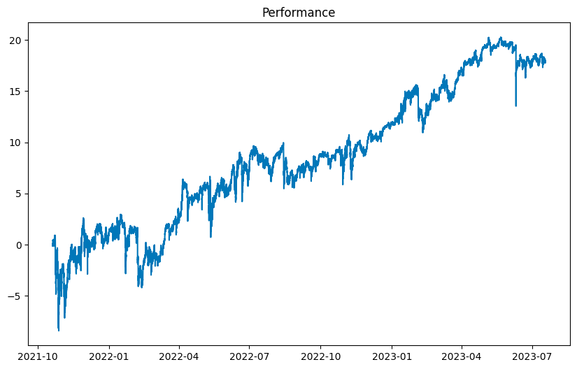
It is important to point out that the simulation thus far is (1) costless and (2) assumes fills at the close of the last candle.

We know from the previous article that doing so effectively means that our trades fill at prices that would be impossible in reality. By doing so, we are likely to observe a highly attractive performance in the simulator, while the same strategy running live would be losing money.

For instance, here is an example strategy that suffers from this problem:

This happens on account of fees and data and market effects such as the bid-ask bounce, latency, spread and market depth, which we currently ignore in our simulation.

In Part 2 we will extend the simulator with:

1. A realistic cost model to make our simulator reflect real life with sufficient accuracy.

2. Funding payments.

3. Support for simulating an arbitrary number of markets at the same time.

Part 2 is for paid subscribers only and can be read here.

Also a quick announcement (I recently have a lot of those):

We’re quickly approaching 500 readers. If you are interested in joining, you can use the link below for a 20% discount until the end of the week.

We regularly publish Quant Infrastructure materials based on systems used in real-life Quant work trading Crypto markets and with source code provided.

Thank you for reading.

(end of Part 1)

1. Disclaimer: Trading is a risky endeavour and I am not responsible for any losses you may incur implementing ideas learnt through these articles.

2. Disclaimer: This article is not financial advice.